Get started

library(dplyr)
library(mrgsim.sa)
library(patchwork)
library(ggplot2)

mrgsim.sa is a package that allows you to do various types of ad-hoc or local sensitivity analysis for models written in mrgsolve. This vignette will help you get started.

By “ad-hoc” sensitivity analysis, I mean selecting some model parameters of interest, varying them at certain discrete, systematic way, simulating from those varied parameters and visualizing the outputs. For example, “what happens when you double the value of a parameter or cut it in half; lets plots outputs for parameters within those two extremes, filling in with 3 or 4 values in between.”

So first, we need a model. This can be any model you write using the mrgsolve package. Here, we’ll use the example house model provided by mrgsolve

mod <- house(outvars = "CP,RESP")

This model has parameters

param(mod)

. 
.  Model parameters (N=14):
.  name value . name  value
.  CL   1     | SEX   0    
.  D1   2     | SEXCL 0.7  
.  F1   1     | SEXVC 0.85 
.  IC50 10    | VC    20   
.  KA   1.2   | WT    70   
.  KIN  100   | WTCL  0.75 
.  KOUT 2     | WTVC  1

and outputs

outvars(mod)

. $cmt
. [1] "RESP"
. 
. $capture
. [1] "CP"

Let’s vary CL and VC and look at the RESP output.

As suggested in the example above, lets double and halve those parameters, and look a total of 5 values between those extremes. Use the parseq_fct() function after selecting the parameters you want to vary

out <- 
  mod %>% 
  ev(amt = 100) %>% 
  parseq_fct(CL, VC, .factor = 2, .n = 5) %>% 
  sens_each()

The “base” value for each parameter is whatever is currently in the model; in this case it is

param(mod)[c("CL", "VC")]

. $CL
. [1] 1
. 
. $VC
. [1] 20

Passing the .factor argument as 2 means multiply those base values by 2 for the upper extreme and 1/2 for the lower extreme. The .n argument says to fill in 5 parameter values between those two extremes.

The sens_each() function call above tells you to vary CL and VC one at a time.

The output is a tibble in long format, with class sens_each

out

.  [38;5;246m# A tibble: 9,680 × 7 [39m
.     case  time p_name p_value dv_name dv_value ref_value
.   [38;5;250m* [39m  [3m [38;5;246m<int> [39m [23m  [3m [38;5;246m<dbl> [39m [23m  [3m [38;5;246m<chr> [39m [23m     [3m [38;5;246m<dbl> [39m [23m  [3m [38;5;246m<chr> [39m [23m       [3m [38;5;246m<dbl> [39m [23m      [3m [38;5;246m<dbl> [39m [23m
.  [38;5;250m 1 [39m     1  0    CL         0.5 RESP       50        50   
.  [38;5;250m 2 [39m     1  0    CL         0.5 RESP       50        50   
.  [38;5;250m 3 [39m     1  0    CL         0.5 CP          0         0   
.  [38;5;250m 4 [39m     1  0    CL         0.5 CP          0         0   
.  [38;5;250m 5 [39m     1  0    CL         0.5 RESP       50        50   
.  [38;5;250m 6 [39m     1  0    CL         0.5 RESP       50        50   
.  [38;5;250m 7 [39m     1  0    CL         0.5 CP          0         0   
.  [38;5;250m 8 [39m     1  0    CL         0.5 CP          0         0   
.  [38;5;250m 9 [39m     1  0.25 CL         0.5 RESP       48.7      48.7 
.  [38;5;250m10 [39m     1  0.25 CL         0.5 CP          1.29      1.29
.  [38;5;246m# ℹ 9,670 more rows [39m

class(out)

. [1] "sens_each"  "tbl_df"     "tbl"        "data.frame"

Taking inventory of this output

count(out, p_name, dv_name)

.  [38;5;246m# A tibble: 4 × 3 [39m
.   p_name dv_name     n
.    [3m [38;5;246m<chr> [39m [23m   [3m [38;5;246m<chr> [39m [23m    [3m [38;5;246m<int> [39m [23m
.  [38;5;250m1 [39m CL     CP        [4m2 [24m420
.  [38;5;250m2 [39m CL     RESP      [4m2 [24m420
.  [38;5;250m3 [39m VC     CP        [4m2 [24m420
.  [38;5;250m4 [39m VC     RESP      [4m2 [24m420

We pass this output object to sens_plot() and name the variable we want to plot

sens_plot(out, "RESP")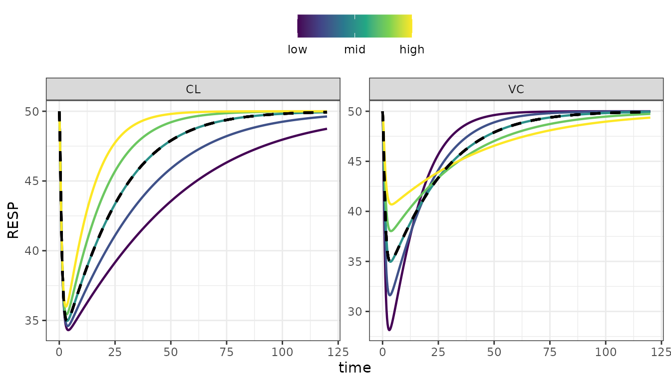

There are other ways to vary parameters in the model

parseq_fct() - increase and decrease by a certain factor
parseq_cv() - increase and decrease by a certain coefficient of variation
parseq_range() - manually specify the range for varying parameters
parseq_manual() - manually specify all values for the parameters

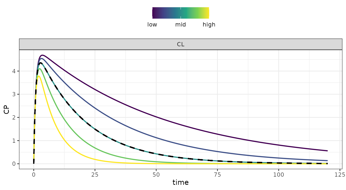
For example, to vary CL by 60% coefficient of variation, plotting 5 values between -2 and 2 sd and looking at CP output

mod %>% 
  ev(amt = 100) %>% 
  parseq_cv(CL, .cv = 50, .nsd = 2) %>% 
  sens_each() %>% 
  sens_plot("CP")

Or we can look at how VC influences approach to steady state

out <- 
  mod %>% 
  ev(amt = 100, ii = 24, addl = 10) %>%
  update(end = 240) %>% 
  parseq_manual(VC = seq(10,100,20)) %>% 
  sens_each()

sens_plot(out, "CP")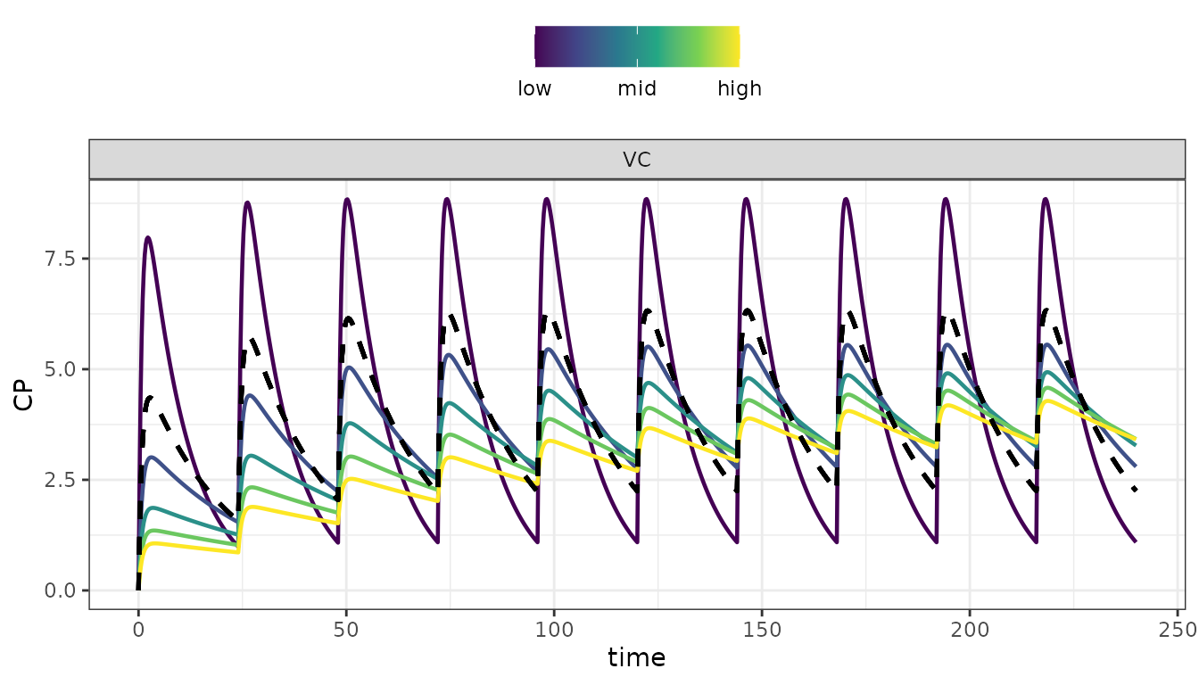

We can also look at multiple outputs on the same plot

out <- 
  mod %>% 
  ev(amt = 100) %>%
  parseq_fct(CL, KA, .n = 4) %>% 
  sens_each(end = 96)

The facet_wrap layout puts parameters in rows and outputs in columns

sens_plot(out, layout = "facet_wrap")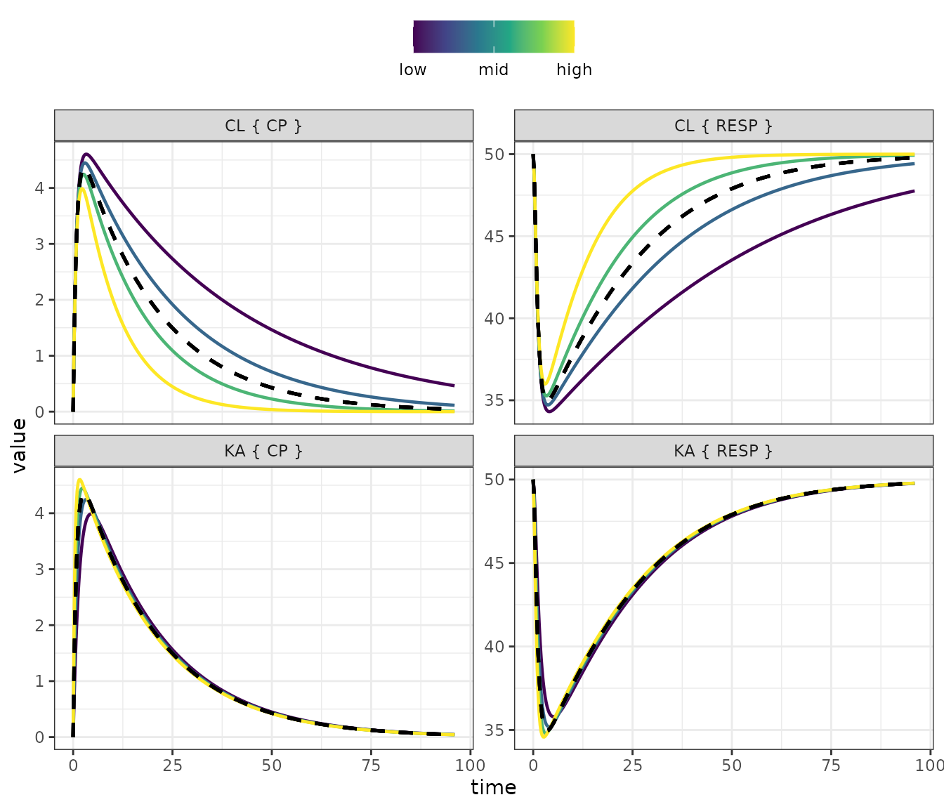

The facet_grid layout puts outputs in rows and parameters in columns

sens_plot(out, layout = "facet_grid")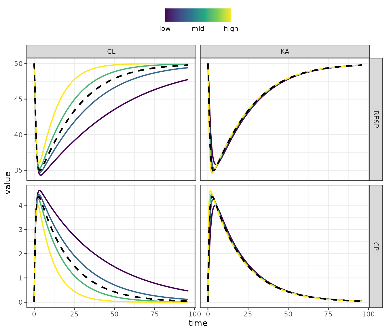

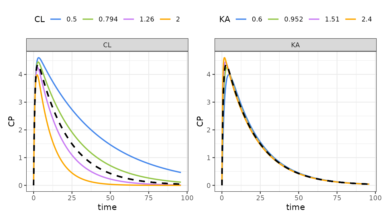
You can also plot this in “grid” format, where the actual parameter values are shown in the legend

sens_plot(out, dv_name = "CP", grid = TRUE)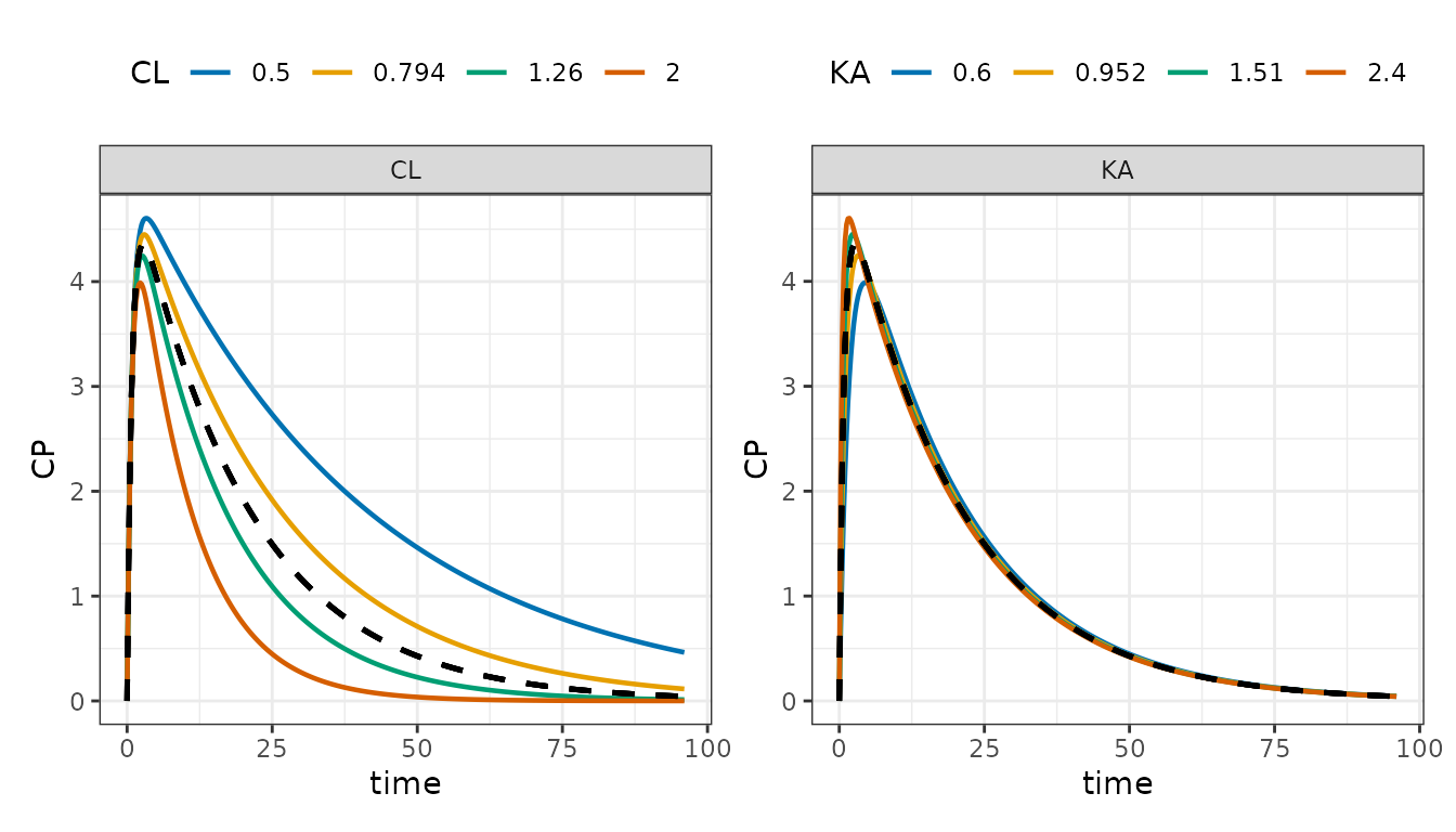

Or look at multiple outputs

out %>% 
  select_sens(dv_name = "RESP,CP") %>% 
  sens_plot(grid = TRUE) %>% 
  patchwork::wrap_plots(ncol = 1)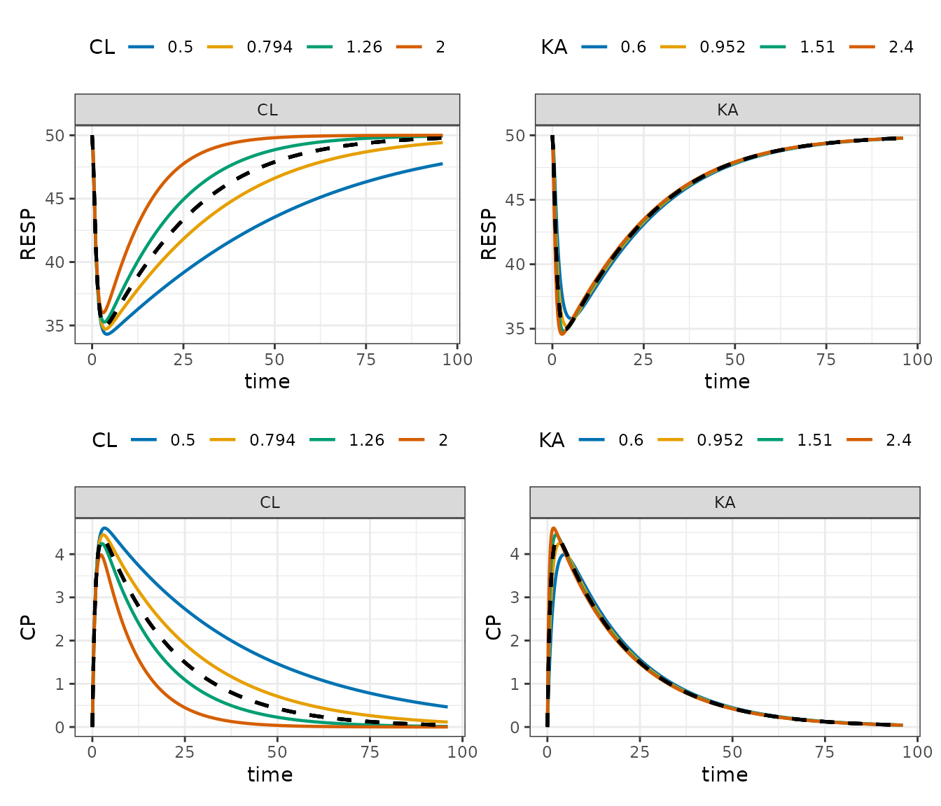

Try a different palette

sens_plot(
  out, 
  "CP", 
  grid = TRUE,
  palette = ggsci::scale_color_atlassian()
)

2026-04-04