A simple, clean workflow for sensitivity analysis with mrgsolve.
param(mod)PK model sensitivity analysis by factor
The nominal (in model) parameter value is divided and multiplied by a factor, generating minimum and maximum bounds for simulating a sequence of parameter values
out <-
  mod %>%
  ev(amt = 100) %>%
  select_par(CL, V) %>%
  parseq_fct(.n=8) %>%
  sens_each()

sens_plot(out, "CP")
The simulated data is returned in a long format
out. # A tibble: 23,232 × 7
. case time p_name p_value dv_name dv_value ref_value
. * <int> <dbl> <chr> <dbl> <chr> <dbl> <dbl>
. 1 1 0 CL 0.5 EV 0 0
. 2 1 0 CL 0.5 EV 0 100
. 3 1 0 CL 0.5 CENT 0 0
. 4 1 0 CL 0.5 CENT 0 0
. 5 1 0 CL 0.5 CP 0 0
. # ℹ 23,227 more rowsAnd you can plot with more informative color scale and legend
sens_plot(out, "CP", grid = TRUE)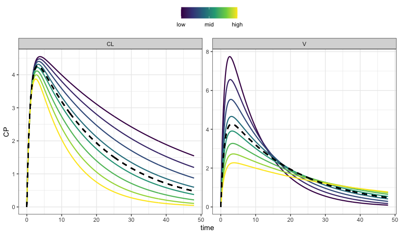
HIV viral dynamic model
We look at latent infected cell pool development over ten years at different “burst” size, or the number of HIV particles released when one cell lyses.
mod <- mread("hiv", "inst/example")
mod %>%
  update(end = 365*10) %>%
  parseq_range(N = c(900,1500), .n = 10) %>%
  sens_each(tscale = 1/365) %>%
  sens_plot("L", grid = TRUE)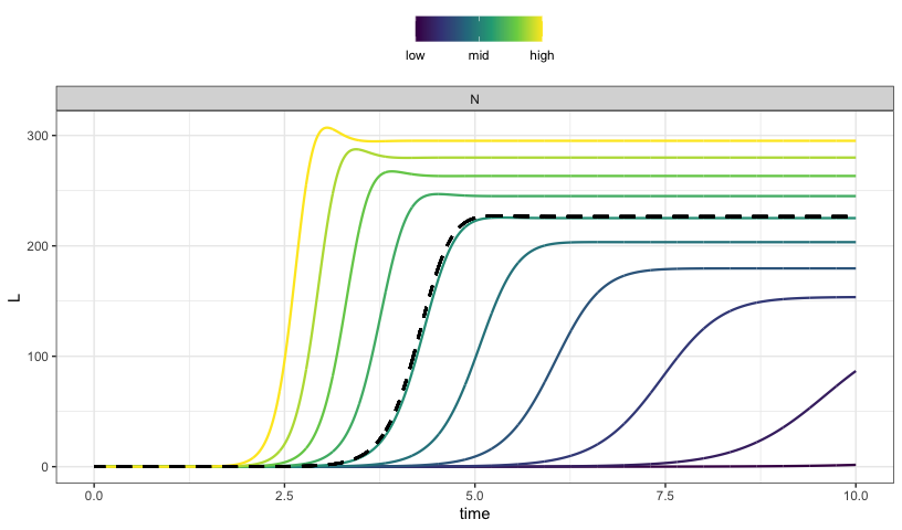
Simulate a grid
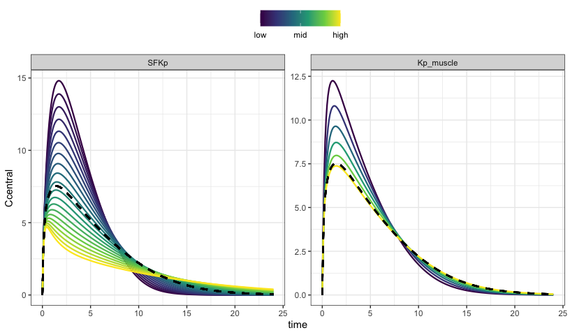
To this point, we have always used sens_each so that each value for each parameter is simulated one at a time. Now, simulate the grid or all combinations.
We use parseq_cv here, which generates lower and upper bounds for the range using 50% coefficient of variation.
out <-
  mod %>%
  update(outvars = "Ccentral") %>%
  ev(amt = 600) %>%
  parseq_cv(fBCLint_all_kg, .n = 7) %>%
  parseq_cv(SFKp, Kp_muscle, .n = 3) %>%
  sens_grid(recsort = 3)

out
. # A tibble: 15,372 × 8
. case fBCLint_all_kg SFKp Kp_muscle time dv_name dv_value ref_value
. * <int> <dbl> <dbl> <dbl> <dbl> <chr> <dbl> <dbl>
. 1 1 0.138 3.65 0.0520 0 Ccentral 0 0
. 2 1 0.138 3.65 0.0520 0 Ccentral 0 0
. 3 1 0.138 3.65 0.0520 0 Ccentral 0 0
. 4 1 0.138 3.65 0.0520 0 Ccentral 0 0
. 5 1 0.138 3.65 0.0520 0.1 Ccentral 3.66 3.14
. # ℹ 15,367 more rows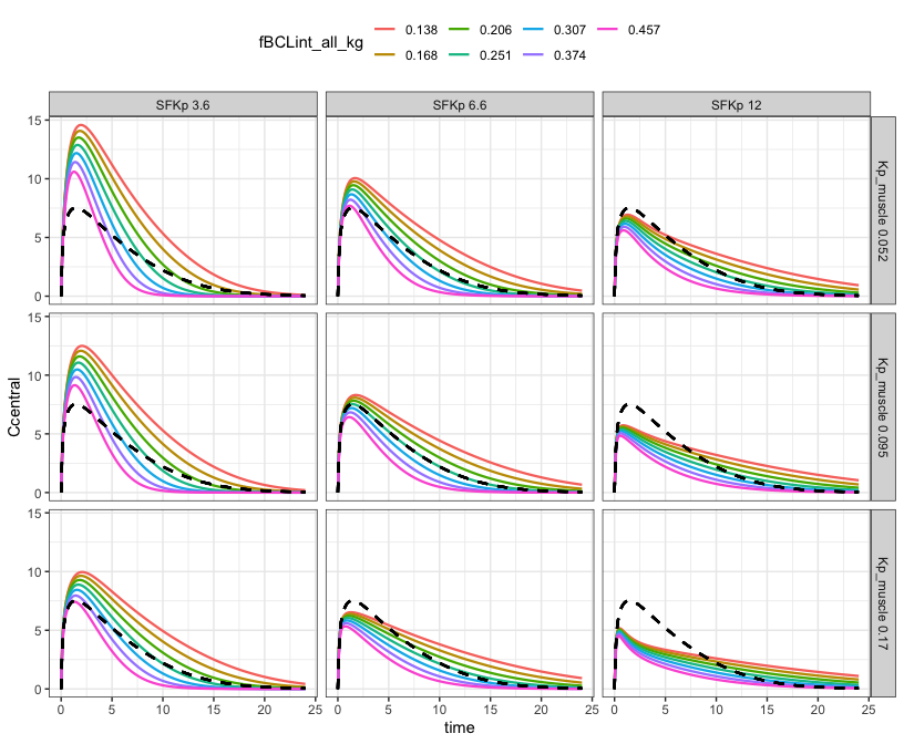
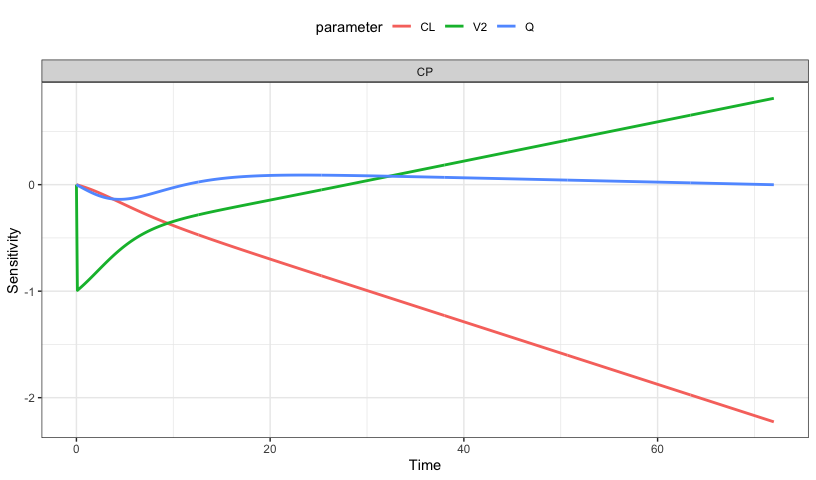
Local sensitivity analysis
mod <- modlib("pk2", delta = 0.1, end = 72). # A tibble: 2,166 × 5
. time dv_name dv_value p_name sens
. <dbl> <chr> <dbl> <chr> <dbl>
. 1 0 CP 0 CL 0
. 2 0 CP 0 CL 0
. 3 0.1 CP 0.472 CL -0.00254
. 4 0.2 CP 0.893 CL -0.00514
. 5 0.3 CP 1.27 CL -0.00782
. # ℹ 2,161 more rows
lsa_plot(out, pal = NULL)