Interact with mrgsimsds objects

Interact with mrgsimsds objects

Usage

# S3 method for class 'mrgsimsds'
dim(x)

# S3 method for class 'mrgsimsds'
head(x, n = 6L, ...)

# S3 method for class 'mrgsimsds'
tail(x, n = 6L, ...)

# S3 method for class 'mrgsimsds'
names(x)

# S3 method for class 'mrgsimsds'
plot(
  x,
  y = NULL,
  ...,
  nid = 16,
  batch_size = 20000,
  logy = FALSE,
  .dots = list()
)

Arguments

x

an mrgsimsds object, output from mrgsim_ds() or as_mrgsim_ds().

n

number of rows to return.

...

arguments to be passed to or from other methods.

y

a formula for plotting simulated data; if not provided, all columns will be plotted.

nid

number of subjects to plot.

batch_size

size of batch when reading data for plot method.

logy

if TRUE, plot data with log y-axis.

.dots

a list of items to pass to mrgsolve::plot_sims().

Details

head() and tail() only look at the first and last file in the data set, respectively, when simulations are stored across multiple files. It is possible this won't correspond to the first and last chunks rows of data you will see when collecting the data via dplyr::collect().

Examples

mod <- house_ds(end = 24)

mod <- omat(mod, diag(0.04, 4))

data <- ev_expand(amt = c(100, 300), ID = 1:20)

set.seed(10203)

out <- mrgsim_ds(mod, data = data)

dim(out)
#> [1] 3920    7
head(out)
#> # A tibble: 6 × 7
#>      ID  time   GUT  CENT  RESP    DV    CP
#>   <dbl> <dbl> <dbl> <dbl> <dbl> <dbl> <dbl>
#> 1     1  0      0     0    70.9  0     0   
#> 2     1  0    100     0    70.9  0     0   
#> 3     1  0.25  68.8  30.9  68.9  1.94  1.94
#> 4     1  0.5   47.3  51.7  65.1  3.24  3.24
#> 5     1  0.75  32.6  65.5  61.1  4.10  4.10
#> 6     1  1     22.4  74.5  57.6  4.66  4.66
tail(out)
#> # A tibble: 6 × 7
#>      ID  time      GUT  CENT  RESP    DV    CP
#>   <dbl> <dbl>    <dbl> <dbl> <dbl> <dbl> <dbl>
#> 1    40  22.8 1.81e-11  124.  39.1  5.57  5.57
#> 2    40  23   1.28e-11  123.  39.2  5.52  5.52
#> 3    40  23.2 9.11e-12  122.  39.4  5.46  5.46
#> 4    40  23.5 6.44e-12  121.  39.5  5.41  5.41
#> 5    40  23.8 4.56e-12  119.  39.7  5.36  5.36
#> 6    40  24   3.23e-12  118.  39.8  5.30  5.30
nrow(out)
#> [1] 3920
ncol(out)
#> [1] 7
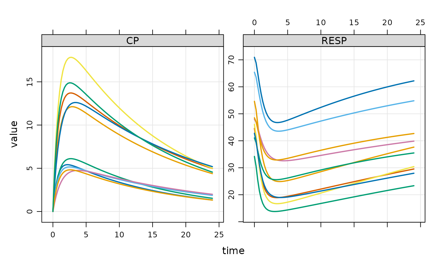
plot(out, ~ CP + RESP, nid = 10)